WIPA Dashboard Guide

Scenarios

The WIPA Scenarios Dashboard is a scenario-only dashboard with a focus on analyzing user’s WIPA predictions — on performance and half‑cycle economics.

Current Dashboard Version: WIPA Scenarios V1.1 (June 11, 2025)

WIPA Scenarios Dashboard Intro

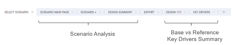
Scenario Analysis

There are 3 core tabs specific to analyzing a user scenario:

1. Scenario Main Page
   Summary of user’s WIPA scenario predictions — metrics specific to month selected.

2. Scenario+
   Summary of user’s WIPA scenario predictions — full curve metrics (PIR10, NPV10).

3. Design Summary
   User-selected well designs (~5 to 10) — summary page.

Additional Details

• Design 1v1 – compare WIPA volumes between two designs (base vs reference).
• Key Drivers – summary of user-selected well design parameters to highlight impact of key drivers.

Scenario Analysis Step-by-Step Guide

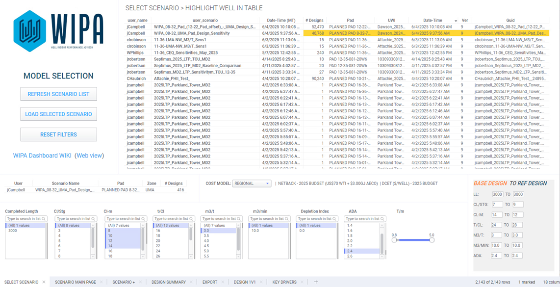
STEP 1: Select Your Scenario

1. Highlight the row in the Scenario Table.
2. Press “Load Selected Scenario.”
3. The design parameters entered upon original input will appear.
4. Users may further filter their design sensitivities.
5. Enter a BASE and REFERENCE (REF) design.
6. Cost model defaults to regional — user may select asset‑specific cost model.

STEP 2: Review WIPA Prediction Outputs

• WIPA data shown will be as‑predicted gas and condensate volumes.
• Select month in the top pane (default = 12mo).
• Enter Flat CGR ○ If the well selected is in ‘Gas Region’ - there will be no WIPA condensate predictions. The user will need to enter a ‘Flat CGR’ in order to estimate condensate volumes. ○ The input for ‘Flat CGR’ is located within the filtering pane at bottom of tab

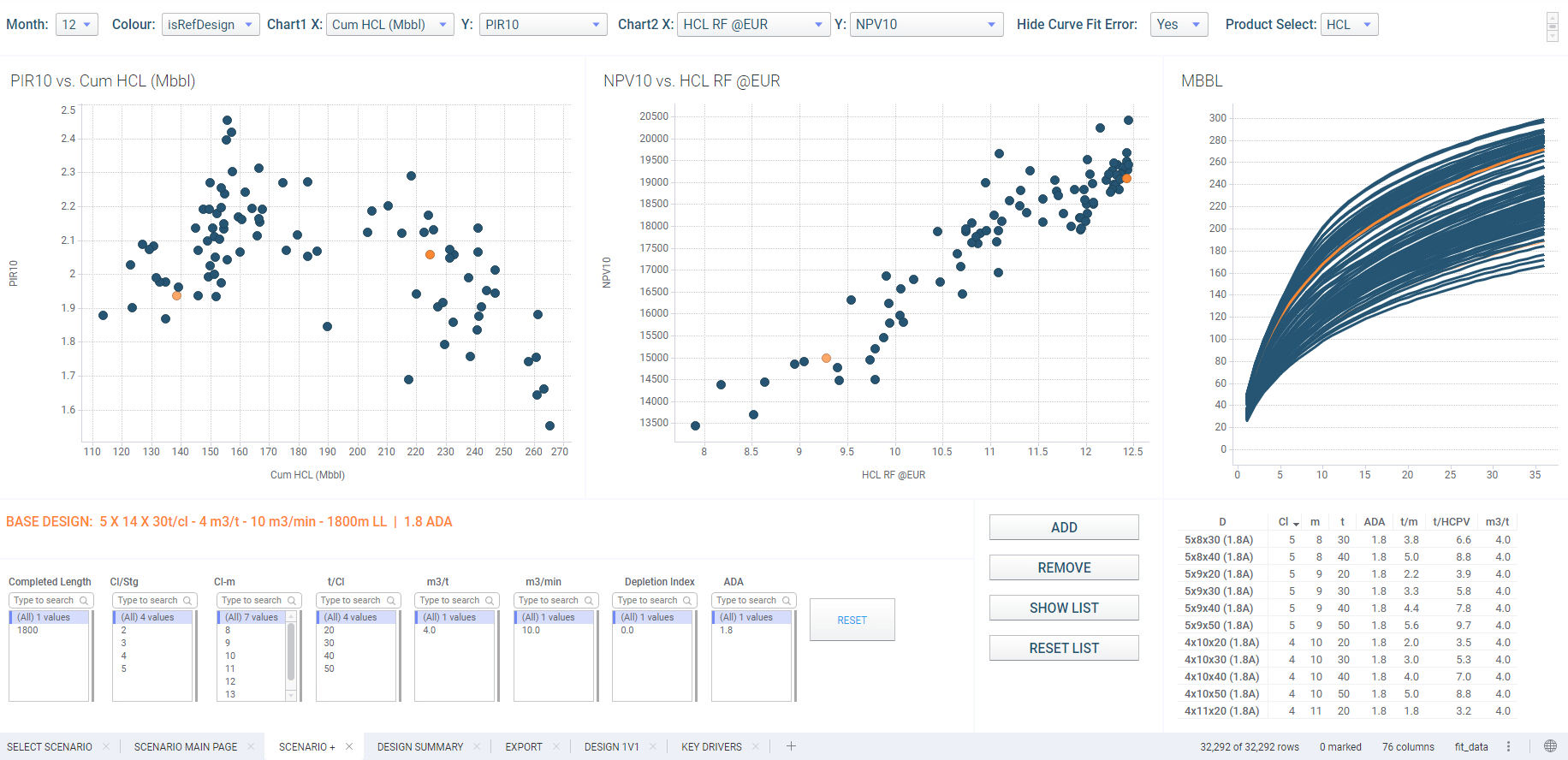
The 2 charts can be changed to plot various scatter plots. Select drop-downs to alter plots

The ‘Color’ drop-down allows user to change how scatter plots are colored. Default is ‘RefDesign’ - which highlights the user-defined base and reference designs

These plots can be colored by well design features - such as Cl/Stg, Cl-m, t/Cl, ADA etc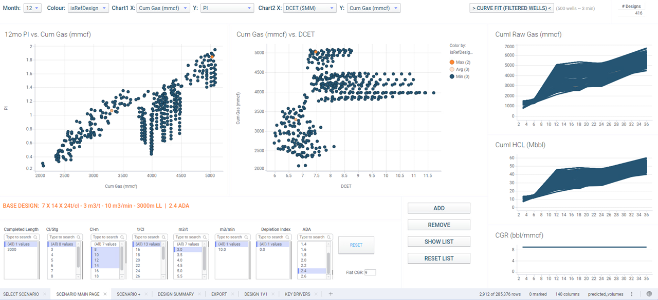

STEP 3: Scenario+

• To populate Scenario+, user must press “Curve Fit” on the main page (top right).

  

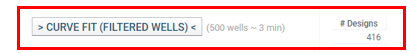
• User should filter wells on the previous page. 500 wells takes 3 min to curve fit

• Page displays curve‑fit gas and condensate volumes.

• Only designs filtered on ‘Main Page’ will be curve-fit and will be shown in Scenario+

• Scenario+ also provides discounted metrics such as NPV10, PIR10, payout ratios.

Overall - this page is a replica of ‘Main Page’ but now has discounted CF metrics such as NPV10, PIR10, Payout ratios etc.

For the final ‘WIPA design summary’ - the user will need to at 5-10 wells to the ‘LIST’ This is done by using the buttons at bottom of tab. (ADD/REMOVE/SHOW/RESET)

ADD - will add the marked designs to list REMOVE - will remove the marked designs from list SHOW - will highlight designs saved in list RESET - will remove all designs from list

Designs can be marked using scatter plots, cum-time curve or table in lower right.

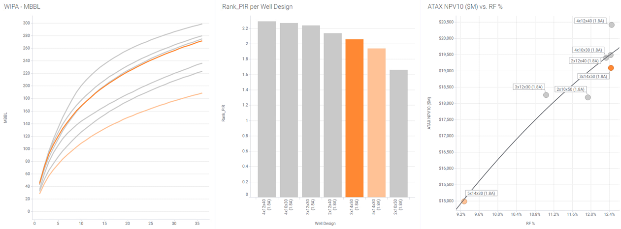
STEP 4: Design Summary

The design summary page includes:

• Cum‑time Curve > color by reference designs
• Bar‑Chart Ranking > User selects ‘Rank-by’ to sort bars by key metric (i.e. NPV10)
• NPV10 vs RF% > Scatter plot with trend line to illustrate NPV and RF% optimization

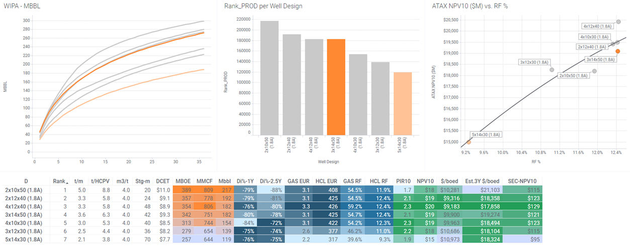
Users can hide the metrics table to enlarge visuals.

Additional Tabs

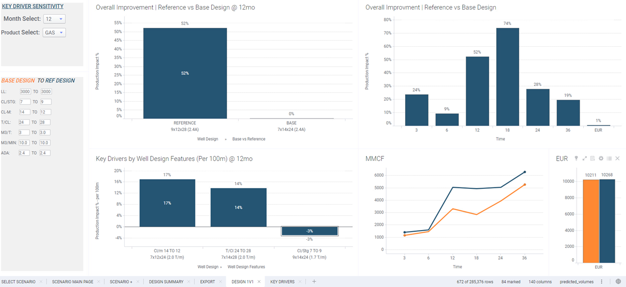
Design 1v1

The Design1V1 tab allows user to compare the WIPA volumes between 2 designs.
Base and Reference designs can be entered by user on this page (or landing page).
Volume metrics will be based on Month and Product dropdowns.

Top Left Chart: % volume difference (Base vs Reference) @ Mo Select
Top Right Chart: % volume difference (Base vs Reference) – All Months + EUR
Bottom Right Chart: Base vs Reference Line Chart
Bottom Left Chart: % Volume difference by Design Parameters

% Volume difference by Design Parameter Examples:

• Cl‑m % is difference between 7x14x24 vs 7x12x24
• t/Cl % is difference between 7x14x24 vs 7x14x28

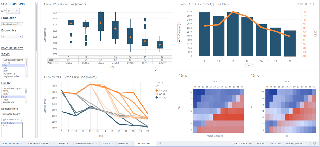
Key Drivers

The Key Drivers tab allows user to summarize WIPA’s performance and economic insights based on user‑selected design parameters (controllable key drivers).

Volume & economic metrics will be based on Month, Product and economic dropdowns.

Top Left Chart: Box Plot → Plots volume by design parameter
Bottom Left Chart: Line Chart → Plots volume by design parameter — line by 2nd parameter
Top Right Chart: Bar Chart w/ Line → Plots volume by design parameter — line by economic metric
Bottom Right Chart: Heat Map → 2 design parameters by volume (left) and economics (right)

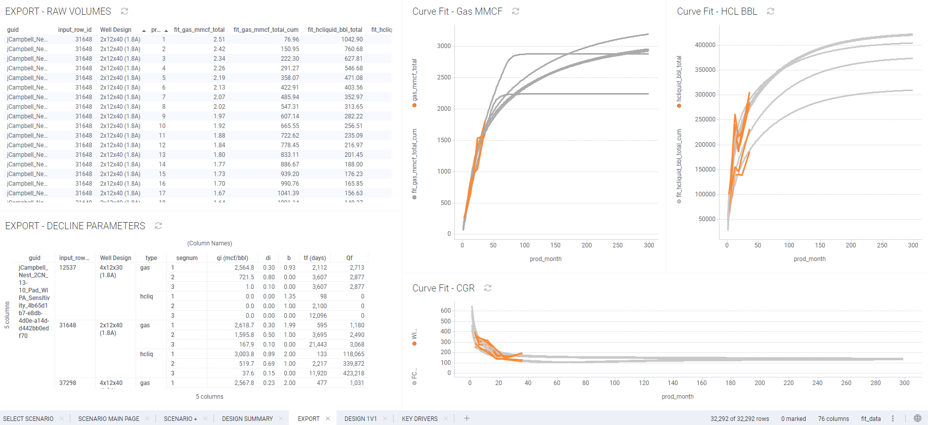
Scenarios Export

Export Tab

Users can export WIPA predictions using the Export tab.
Only wells added to the final Design Summary List are available for export.

EXPORT – Raw Volumes

• Raw Monthly volumes - up to 300 months - are available to export.
• Rate (mmcf/d, bbl/d), Cum (mmcf,bbl)
• ML Prediction (gas_mmcf and hcliquid_bbl) are provided as reference.

EXPORT – Decline Parameters

• Segment parameters used in curve fit for gas and hcliquid can be exported.

Exported data can then be used as volumetric inputs in Mosaic for further economic analysis

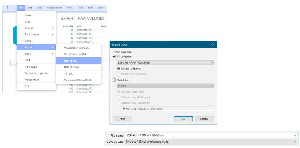
How to Export Tables

To export the 2 tables (EXPORT - RAW VOLUMES or EXPORT - DECLINE PARAMETERS)

• Select table to export
• Select File > Export > Data to file…
• Select ‘Export data from: Visualization (should be selected by default)
  • Ensure table is selected table to export
• Select ‘Ok’
• Save file in user-defined directory (file type should be .csv or .xls)